Introduction to Elmasri et al.(2020) Host-Parasite Link Prediction Package
Maxwell J. Farrell & Mohamad Elmasri
April 28 2020
Source:vignettes/HPprediction.Rmd
HPprediction.RmdData
To begin we will use a subsection of the GMPD 2.0 and the associated Mammal supertree updated by Fritz et al. 2009
data(gmpd)
data(mammal_supertree)

# Removing parasites not reported to species
gmpd <- gmpd[grep("sp[.]",gmpd$ParasiteCorrectedName, invert=TRUE),]
gmpd <- gmpd[grep("not identified",gmpd$ParasiteCorrectedName, invert=TRUE),]

# Subsetting host family Bovidae
gmpd <- gmpd[gmpd$HostFamily=="Bovidae",]

# Formatting host names to match phylogeny
gmpd$HostCorrectedName <- gsub(" ","_", gmpd$HostCorrectedName)

# Creating binary interaction matrix
com <- table(gmpd$HostCorrectedName, gmpd$ParasiteCorrectedName)
com[com>1] <- 1
com <- as.matrix(unclass(com), nrow=nrow(com), ncol=ncol(com))

# loading phylogeny and pruning to hosts in the interaction matrix
mammal_supertree <- drop.tip(mammal_supertree, mammal_supertree$tip.label[!mammal_supertree$tip.label%in%rownames(com)])

# merge the tree and interaction matrix
cleaned <- network_clean(com, mammal_supertree, 'full')
#> Warning: not all rows in Z exist tree; missing are removed from Z!
#> [1] "Z has empty columns - these have been removed!"
#> [1] "ordering the rows of Z to match tree..."
#> [1] "normalizing tree edges by the maximum pairwise distance!"
com <- cleaned$Z                         # cleaned binary interaction matrix
tree <- cleaned$tree                     # cleaned tree
Plotting Input Data
To visualize the structure of the input interaction matrix we can use two built-in plotting functions.
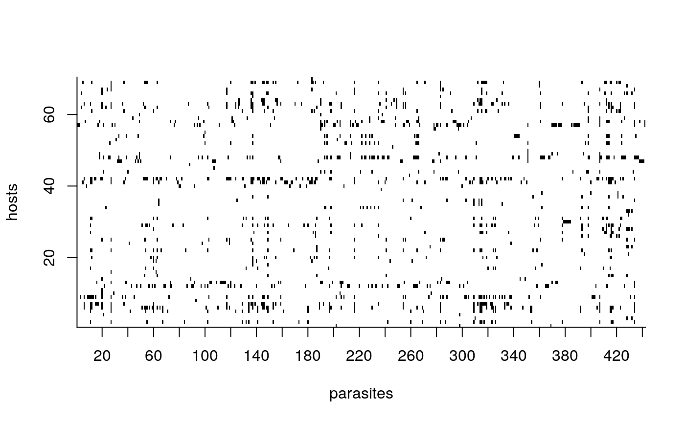
We can also use the function lof to left order the interaction matrix before plotting:
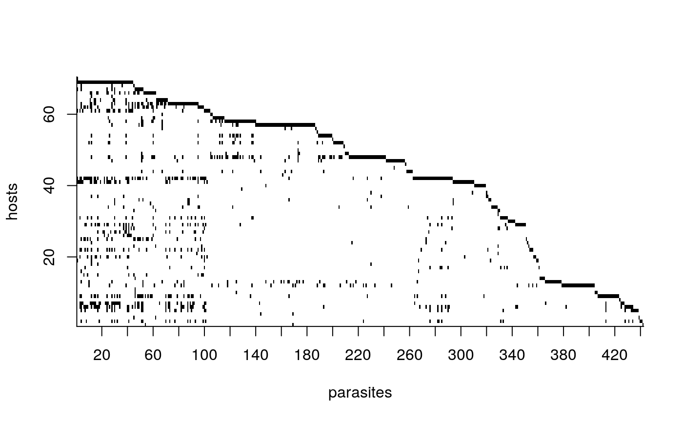
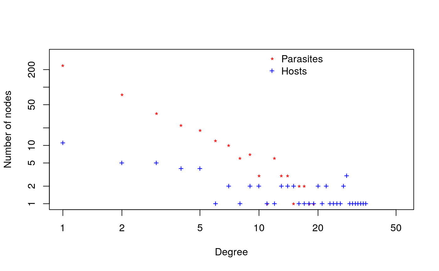
Another interesting property of networks to explore is the degree distribution. We can look at the degree distribution for both hosts and parasites with the following function:
Running the model
Running for 1500 slices (iterations) on an i7-6560U and 16GB RAM took about 25 seconds.
out <- network_est(Z = com, tree = tree, slices = 1000, model.type = 'full')
#> [1] "Running full model..."
#> [1] "Run for 1000 slices with 500 burn-ins"
#> [1] "Matrix dimension: 70 x 442"
#> [1] "slice: 200, at 2020-04-28 21:43:02"
#> [1] "slice: 400, at 2020-04-28 21:43:08"
#> [1] "slice: 600, at 2020-04-28 21:43:15"
#> [1] "slice: 800, at 2020-04-28 21:43:21"
#> [1] "slice: 1000, at 2020-04-28 21:43:28"
#> [1] "Done!"
str(out)
#> List of 3
#>  $ param:List of 6
#>   ..$ w      : num [1:442, 1:500] 1.259 1.248 0.621 1.097 1.335 ...
#>   ..$ y      : num [1:70, 1:500] 0.441 11.398 1.097 3.013 6.011 ...
#>   ..$ eta    : num [1:500] 8.11 7.4 8.54 8.54 7.98 ...
#>   ..$ g      : NULL
#>   ..$ burn.in: num 500
#>   ..$ sd     :List of 3
#>   .. ..$ w  : num [1:442] 1.96 2 2.14 1.98 2.05 ...
#>   .. ..$ y  : num [1:70] 1.35 6.95 2.27 3.27 4.99 ...
#>   .. ..$ eta: num 0.808
#>  $ Z    : num [1:70, 1:442] 0 0 0 0 0 0 0 0 0 0 ...
#>   ..- attr(*, "dimnames")=List of 2
#>   .. ..$ : chr [1:70] "Addax_nasomaculatus" "Oryx_gazella" "Hippotragus_equinus" "Hippotragus_niger" ...
#>   .. ..$ : chr [1:442] "Acinetobacter lwoffii" "Actinobacillus actinomycetemcomitans" "Africanostrongylus buceros" "Agriostomum cursoni" ...
#>  $ tree :List of 4
#>   ..$ edge       : int [1:118, 1:2] 71 72 73 74 75 76 76 75 77 77 ...
#>   ..$ edge.length: num [1:118] 0.1774 0.0604 0.0792 0.3736 0.0604 ...
#>   ..$ Nnode      : int 49
#>   ..$ tip.label  : chr [1:70] "Addax_nasomaculatus" "Oryx_gazella" "Hippotragus_equinus" "Hippotragus_niger" ...
#>   ..- attr(*, "class")= chr "phylo"
#>   ..- attr(*, "order")= chr "cladewise"
Example traceplots
# Affinity parameter of parasite 1
plot(out$param$w[1,],type="l", col=2, ylab="Affinity parameter for parasite 1", xlab="Iteration")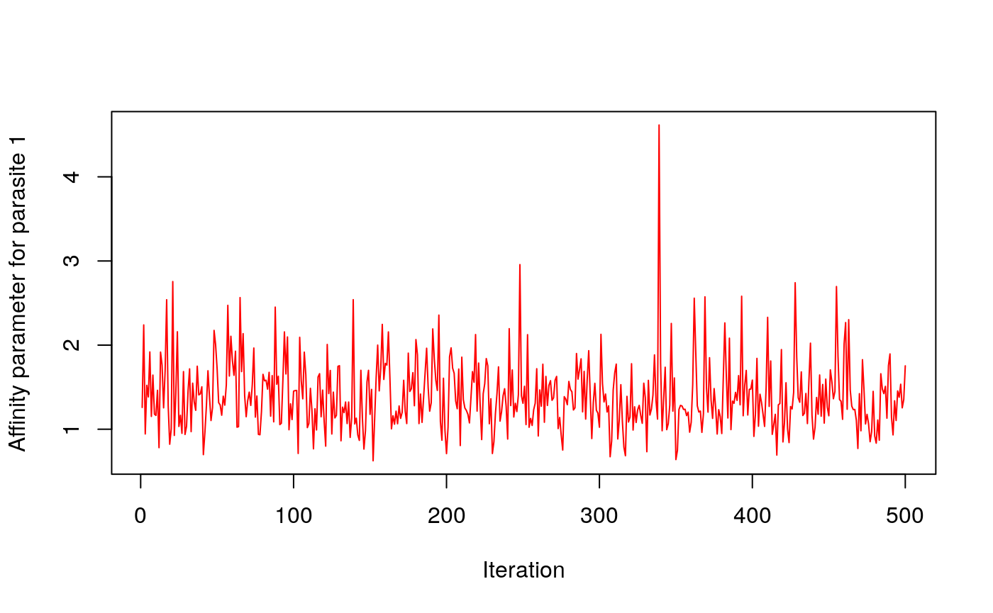
# Affinity parameter of host 1
plot(out$param$y[1,],type="l", col=4, ylab="Affinity parameter for host 1", xlab="Iteration")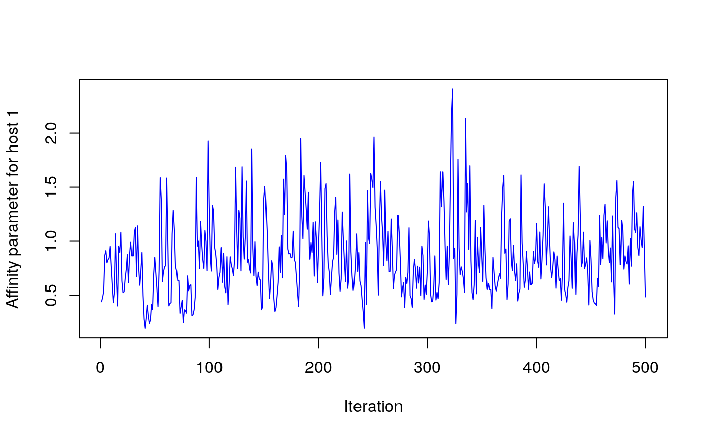
# Phylogeny scaling parameter
plot(out$param$eta, type="l",col="darkgreen", ylab="Phylogeny scaling parameter (EB model)", xlab="Iteration")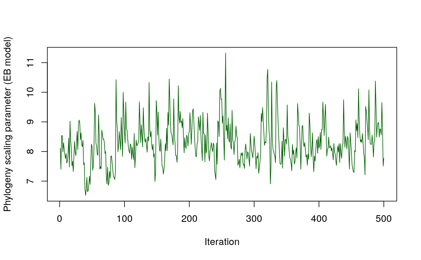
Identfying top predicted links with no documentation
topPairs(P, out$Z)
#>                          Hosts                                Parasites
#> 22003      Rupicapra_rupicapra                    Rhipicephalus evertsi
#> 28449       Aepyceros_melampus                        Toxoplasma gondii
#> 27819       Aepyceros_melampus                Teladorsagia circumcincta
#> 29073      Rupicapra_rupicapra              Trichostrongylus falculatus
#> 16409       Aepyceros_melampus                    Nematodirus spathiger
#> 19763      Rupicapra_rupicapra Pestivirus Bovine viral diarrhea virus 1
#> 1843       Rupicapra_rupicapra                       Bacillus anthracis
#> 28835 Tragelaphus_strepsiceros                    Trichostrongylus axei
#> 10383      Rupicapra_rupicapra                     Impalaia tuberculata
#> 27855 Tragelaphus_strepsiceros                Teladorsagia circumcincta
#>               p
#> 22003 0.4950395
#> 28449 0.4809607
#> 27819 0.4697782
#> 29073 0.4515099
#> 16409 0.4427870
#> 19763 0.4418728
#> 1843  0.4289917
#> 28835 0.4251196
#> 10383 0.4174443
#> 27855 0.4051877
General approach to running the model with 5-fold cross validation
## General variables
MODEL = 'full'                       # full, distance or affinity
SLICE = 1000                          # no of iterations
NO.CORES = 3                         # maximum cores to use
COUNT = TRUE                         # TRUE = count data, FALSE = year of first pub.
ALPHA.ROWS = 0.3                     # hyperparameter for prior over rows affinity, effective under affinity and full models only
ALPHA.COLS = 0.3                     # hyperparameter for prior over columns affinity, effective under affinity and full models only

## Loading required packages
require(parallel)

## preparing tree and com
cleaned <- network_clean(com, tree, 'full')
com <- cleaned$Z                         # cleaned binary interaction matrix
tree <- cleaned$tree                     # cleaned tree

## indexing 5-folds of interactions
folds <- cross.validate.fold(com, n= 5, min.per.col=2)
[1] "Actual cross-validation rate is 0.095"
[2] "Actual cross-validation rate is 0.095"
[3] "Actual cross-validation rate is 0.095"
[4] "Actual cross-validation rate is 0.095"
[5] "Actual cross-validation rate is 0.096"

# returns a matrix of 3 columns (row, col, group), (row, col) correspond to Z, group to the CV group
tot.gr <- length(unique(folds[,'gr']))   # total number of CV groups

## A loop to run over all CV groups
res <- mclapply(1:tot.gr, function(x, folds, Z, tree, slice, model.type, ALPHA.ROWS, ALPHA.COLS){

    ## Analysis for a single fold
    Z.train = Z
    Z.train[folds[which(folds[,'gr']==x),c('row', 'col')]]<-0

    ## running the model of interest
    obj = network_est(Z.train, slices=slice, tree=tree, model.type=model.type,
                      a_y = ALPHA.ROWS, a_w = ALPHA.COLS)

    P = sample_parameter(obj$param, model.type, Z.train, tree)
    Eta = if(is.null(obj$param$eta)) 0 else mean(obj$param$eta)

    ## order the rows in Z.test as in Z.train
    roc = rocCurves(Z, Z.train, P, plot=FALSE, bins=400, all=FALSE)
    tb  = ana.table(Z, Z.train, P, roc,  plot=FALSE)
    roc.all = rocCurves(Z, Z.train, P=P, plot=FALSE, bins=400, all=TRUE)
    tb.all  = ana.table(Z, Z.train, P, roc.all, plot=FALSE)

    list(param=list(P=P, Eta = Eta), tb = tb,
         tb.all = tb.all, FPR.all = roc.all$roc$FPR,
         TPR.all=roc.all$roc$TPR, FPR = roc$roc$FPR, TPR=roc$roc$TPR)

},
    folds=folds, Z = com, tree=tree, model.type=MODEL, slice = SLICE,
    ALPHA.ROWS = ALPHA.ROWS, ALPHA.COLS= ALPHA.COLS,
    mc.preschedule = TRUE, mc.cores = min(tot.gr, NO.CORES))
[1] "Running full model..."
[1] "Running full model..."
[1][1] "Running full model..."
 "Run for 1000 slices with 500 burn-ins"
[1] "Matrix dimension: 70 x 442"
[1] "Run for 1000 slices with 500 burn-ins"
[1] "Matrix dimension: 70 x 442"
[1] "Run for 1000 slices with 500 burn-ins"
[1] "Matrix dimension: 70 x 442"
[1] "slice: 200, at 2020-04-18 18:08:37"
[1] "slice: 200, at 2020-04-18 18:08:37"
[1] "slice: 200, at 2020-04-18 18:08:37"
[1] "slice: 400, at 2020-04-18 18:08:41"
[1] "slice: 400, at 2020-04-18 18:08:41"
[1] "slice: 400, at 2020-04-18 18:08:41"
[1] "slice: 600, at 2020-04-18 18:08:45"
[1] "slice: 600, at 2020-04-18 18:08:45"
[1] "slice: 600, at 2020-04-18 18:08:45"
[1] "slice: 800, at 2020-04-18 18:08:51"
[1] "slice: 800, at 2020-04-18 18:08:51"
[1] "slice: 800, at 2020-04-18 18:08:51"
[1] "slice: 1000, at 2020-04-18 18:08:57"
[1] "Done!"
[1] "slice: 1000, at 2020-04-18 18:08:57"
[1] "Done!"
[1] "slice: 1000, at 2020-04-18 18:08:58"
[1] "Done!"
[1] "Running full model..."
[1] "Run for 1000 slices with 500 burn-ins"
[1] "Matrix dimension: 70 x 442"
[1] "Running full model..."
[1] "Run for 1000 slices with 500 burn-ins"
[1] "Matrix dimension: 70 x 442"
[1] "slice: 200, at 2020-04-18 18:09:07"
[1] "slice: 200, at 2020-04-18 18:09:07"
[1] "slice: 400, at 2020-04-18 18:09:12"
[1] "slice: 400, at 2020-04-18 18:09:12"
[1] "slice: 600, at 2020-04-18 18:09:18"
[1] "slice: 600, at 2020-04-18 18:09:19"
[1] "slice: 800, at 2020-04-18 18:09:25"
[1] "slice: 800, at 2020-04-18 18:09:26"
[1] "slice: 1000, at 2020-04-18 18:09:32"
[1] "Done!"
[1] "slice: 1000, at 2020-04-18 18:09:32"
[1] "Done!"
We can analyze the performance of the model via the area under the receiver operating characteristic curve (AUC), and the proportion of 1s in the original data successfully recovered.
#> Loading required package: parallel#> m.auc m.pred.held.out.ones m.thresh m.hold.out
#> 1 0.9249 87.17949 0.04260652 117
#> 2 0.9211 88.03419 0.05263158 117
#> 3 0.9380 90.59829 0.04511278 117
#> 4 0.9258 84.61538 0.05764411 117
#> 5 0.9445 92.37288 0.04761905 118
#> [1] "Model: full, AUC: 0.930860 and percent 1 recovered from held out: 88.560046"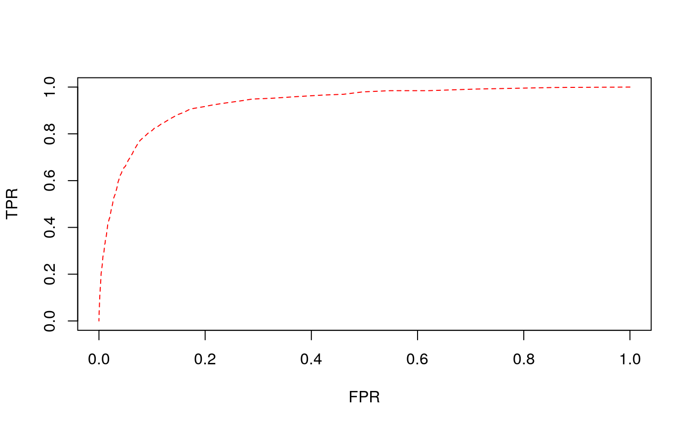
We can also construct the posterior probability matrix ‘P’ as the average across each fold, and look at the top undocumented interactions.
## Constructing the P probability matrix from CV results
P = matrix(rowMeans(sapply(res, function(r) r$param$P)),
    nrow = nrow(com), ncol = ncol(com))

## left ordering of interaction and probability matrix
indices = lof(com, indices = TRUE)
com = com[, indices]
P = P[, indices]
rownames(P)<-rownames(com)
colnames(P)<-colnames(com)

## view top undocumented interactions
topPairs(P,1*(com>0),topX=10)
#>                         Hosts                                Parasites
#> 2053      Rupicapra_rupicapra                    Rhipicephalus evertsi
#> 3529       Aepyceros_melampus                        Toxoplasma gondii
#> 2823      Rupicapra_rupicapra              Trichostrongylus falculatus
#> 4159       Aepyceros_melampus                Teladorsagia circumcincta
#> 1913      Rupicapra_rupicapra Pestivirus Bovine viral diarrhea virus 1
#> 1709       Aepyceros_melampus                    Nematodirus spathiger
#> 233       Rupicapra_rupicapra                       Bacillus anthracis
#> 1143      Rupicapra_rupicapra                     Impalaia tuberculata
#> 2725 Tragelaphus_strepsiceros                    Trichostrongylus axei
#> 6645 Tragelaphus_strepsiceros           Trichostrongylus colubriformis
#>              p
#> 2053 0.4775287
#> 3529 0.4562461
#> 2823 0.4515121
#> 4159 0.4496634
#> 1913 0.4429673
#> 1709 0.4394255
#> 233  0.4210100
#> 1143 0.4160180
#> 2725 0.4133397
#> 6645 0.3945742
We can also compare the input matrix to the posterior interaction matrix, and the orginal phylogeny compared to the phylogeny with estimated EB scaling.
par(mfrow=c(1,2))

## printing input Z
plot_Z(com, tickMarks=20)

## printing posterior interaction matrix
plot_Z(1*(P > mean(sapply(res, function(r) r$tb$thres))), tickMarks=20)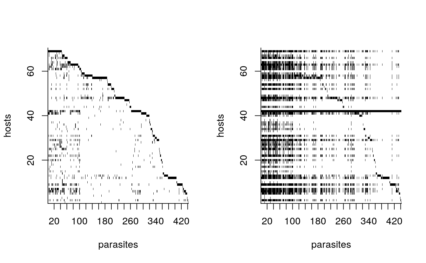
## printing input tree
plot(tree, show.tip.label=FALSE)

## printing output tree
if(grepl('(full|dist)', MODEL)){
    Eta = mean(sapply(res, function(r) r$param$Eta))
    print(paste('Eta is', Eta))
    plot(rescale(tree, 'EB', Eta), show.tip.label=FALSE)
}
#> [1] "Eta is 6.83615118463669"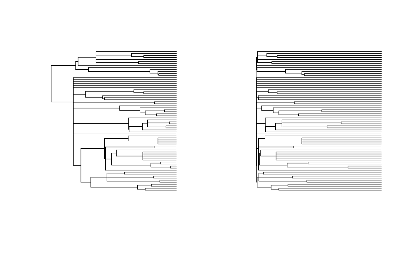
References
Elmasri, M., Farrell, M. J., Davies, T. J., & Stephens, D. A. (2020). A hierarchical Bayesian model for predicting ecological interactions using scaled evolutionary relationships. Annals of Applied Statistics, 14(1), 221-240.