Introduction to traveltimeHMM: making reliable travel time predictions on road networks
Mohamad Elmasri, Aurélie Labbe, Denis Larocque, Laurent Charlin and Éric Germain
2020-11-25
Source:vignettes/traveltimeHMM.Rmd
traveltimeHMM.RmdIntroduction
In the new world of data, decision-making is becoming more data-driven then ever. This is increasingly true for urban transportation, where the ubiquitous expected time of arrival (ETA) is heavily used. Providing reliability measure for ETA’s is likely to improve our understanding of travel time and to provide systems with better decision-making metrics. This traveltimeHMM package provides various methods to estimate the distribution of travel time on a given route, by leveraging GPS data from moving vehicles on road segments, with flexible temporal binning.
Implemented methods include the proposed TRIP model (and its variates) in Woodard et. al. (2016). Other methods are in the pipeline.
This is a work in progress. For bugs and features, please refer to here.
Example data set: tripset
This package includes a small data set (tripset) that aggregates map-matched anonymized mobile phone GPS data collected in Quebec city in 2014 using the Mon Trajet smartphone application developed by Brisk Synergies Inc. The precise duration of the time period is kept confidential.
tripset is used to explore methods offered in this package. Data similar to tripset can be generated using other sources of GPS data, however, a preprocessing stage is necessary to map-match and aggregate the information up to the road segment (link) level. Such preprocessing is already performed on tripset.
traveltimeHMM does not perform this preprocessing stage, and the software cannot make use of raw GPS data.
library(traveltimeHMM)
data(tripset)
head(tripset)
#>   tripID linkID timeBin logspeed traveltime    length                time
#> 1   2700  10469 Weekday 1.692292  13.000000  70.61488 2014-04-28 06:07:27
#> 2   2700  10444 Weekday 2.221321  18.927792 174.50487 2014-04-28 06:07:41
#> 3   2700  10460 Weekday 2.203074   8.589937  77.76295 2014-04-28 06:07:58
#> 4   2700  10462 Weekday 1.924290  14.619859 100.15015 2014-04-28 06:08:07
#> 5   2700  10512 Weekday 1.804293   5.071986  30.81574 2014-04-28 06:08:21
#> 6   2700   5890 Weekday 2.376925  31.585355 340.22893 2014-04-28 06:08:26
Travel data is organized around the notions of trips and links. Links are road segments each with well-defined beginning and end points and which can be traversed. A vehicle performs a trip when it travels from a start point to an end point through a sequence of links. Thus trips can be considered as ordered sequences of links. tripset includes data for a collection of trips.
Field
tripIDcontains each trip’s ID, whereas fieldlinkIDcontains the IDs of each link making up a trip. Both fields need to be numerical. It is assumed that, in the data set, all trips are grouped together and all links of a given trip appear in the order in which they are traversed (No verification is performed to that effect). A given link corresponds to some physical entity such as a road segment, a portion of a road segment, or any combination of those. Hence, it is expected that links are used in more than one trip.Field
timeBin(character string, or factor) refers to the time “category” when the traversal of a given link occurred. Time bins should reflect as much as possible time periods of the week encompassing similar traffic classes. Intripsetwe define five time bins:Weekday,MorningRush,EveningRush,EveningNightandWeekendday.
| Period of the week | Time bin |
|---|---|
| Mon - Fri outside rush hour | Weekday |
| Mon - Fri, 7AM - 9AM | MorningRush |
| Mon - Fri, 3PM - 6PM | EveningRush |
| Sat 9AM - 9PM + Sun 9AM - 7PM | Weekendday |
| Sat - Sun otherwise | EveningNight |
Field
logspeedcontains the natural logarithm of the speed (in meter/second) of traversal of each link. This information is central to the estimation algorithm.Field
traveltimerefers to the traversal time (in seconds) of each link. This field is mostly for reference and is not used directly in the package.Field
lengthrefers to the length (in meters) of each link. This information is used by the prediction algorithm.Field
timegives the entry time in POSIXct format for the traversal of a given link. Individual datums are not used directly; however, the start time of the very first traversal is likely to be useful for providing the start time of a whole trip to the prediction function. Fieldtimedetermine the time bin for each link, as illustrated in Table 1.
traveltimeHMM includes functionality to convert time stamps to alternative time bins, please refer to Time bins.
Statistical models
At the core of traveltimeHMM is a statistical model that aims to approximate the distribution of travel time over a combination of links and a start time, on the basis of data just like that we just described. traveltimeHMM includes multiple models, including the ones in Woodard et. al. (2016). The following sections describe each model implementation.
Woodard Models
Woodard et. al. (2016) models are built around an HMM construction. The most general model is the trip-HMM, which estimates the mean and standard deviation of the speed for each combination of road link, time bin, and congestion state. This latter concept involve defining a finite number of hidden states that reflect traffic fluidity of a trip at a given place and time. For instance the fact that one is driving downtown during rush hour (or not), they might (or might not) fall into congestion at a specific link and time. Hence, congestion level as a property of the individual trip, rather than a property of the link and time. In our example, we chose to define two congestion states which we implicitly call “congested” and “not-congested”.
In order to deal properly with the fact that the congestion states are unobserved, the model estimates parameters for each hidden state. These estimates are computed using a Markov model and Viterbi forward-backward algorithm. To capture variability in speed due to trip-specific conditions (e.g. driver habits), the model also estimates a random trip effect.
Let \(T_{i,k}\) be the travel time of trip \(i\) on road \(R_k\), here \(R_k\) is the unique road in the map representing the \(k\)-th traversed road on the travel path of trip \(i\), such that
\[T_{i,k} = \frac{d_{i,k}}{E_iS_{i,k}}, \quad i \in I, k \in \{1, \dots, n_i\},\]
where \(S_{i,k}\) is the trip’s \(i\) speed on link \(k\) of length \(d_{i,k}\), and \(E_i\) is the driver specific random effect, which is modelled as
\[\log E_i \sim N(0, \tau^2).\]
The speed distribution is modelled as a log-normal, with parameters \(\mu\) and \(\sigma\), as \[\log S_{i,k}\mid Q_{i,k} \sim N( \mu_{R_{i,k}, b_{i,k}, Q_{i,k}}, \sigma^2_{R_{i,k}, b_{i,k}, Q_{i,k}}) , \quad \text{with} \quad \mu_{j,b,q-1} \leq \mu_{j,b,q}\] where \(N\) is the normal distribution, and \(Q_{i,k}\) is a hidden state representing congestion, \(b_{i,k} \in B\) is a set of time bins on link \(k\).
The transition states are defined as \[P(Q_{i,1}=q) = \gamma_{R_{i,1}, b_{i,1}} (q)\] \[P (Q_{i,k}= q \mid Q_{i,k-1}=q') = \Gamma_{R_{i,k}, b_{i,k}} (q',q)\]
Variants
The other three models are special cases of trip-HMM described above.
The HMM model, which is the default, assumes that the trip effect is fixed to 1 (\(E_i=1\)). The trip model considers the existence of a single traffic state (does not use the hidden states abstraction); under this model the parameters \(\gamma\) and \(\Gamma\) remain undefined. Finally, the no-dependence model is the most basic of the four, assumes no trip effect and no hidden Markov states. Table 2 provides a summary of the characteristics of each model.
| Model type |
Hidden Markov model (HMM)
|
Trip effect model (trip)
|
|---|---|---|
| trip-HMM | YES | YES |
| HMM (default) | YES | NO |
| trip | NO | YES |
| no-dependence | NO | NO |
Model estimation
Model estimation is performed using Algorithm 1 of Woodard et al. (2016) The estimation algorithm takes input data on speeds (on a logarithmic scale), trips, road links and time periods, and calculates a set of parameter estimates for a specified model.
Calculations are performed iteratively as is typical of non-linear optimization algorithms. The estimates for each parameter are updated at each iteration, and the algorithm stops when either the variation in parameter estimates between two successive iterations is below a predefined threshold value, or a predefined maximum number of iterations is reached.
Calling traveltimeHMM
The estimation algorithm can be executed by calling the traveltimeHMM function. The function’s interface is as follows.
traveltimeHMM(logspeeds = NULL,
              trips = NULL,
              timeBins = NULL,
              linkIds = NULL,
              data = NULL,
              nQ = 1L,
              model = c("HMM", "trip-HMM", "trip", "no-dependence"),
              tol.err = 10,
              L = 10L,
              max.it = 20,
              verbose = FALSE,
              max.speed = NULL,
              seed = NULL,
              tmat.p = NULL,
              init.p = NULL)
traveltimeHMM can be called either using explicit parameters or using a composite object incorporating the main parameters, for example, a data.frame.
Explicit calling is as
fit <- traveltimeHMM(logspeeds = tripset$logspeed,
                     trips = tripset$tripID,
                     timeBins = tripset$timeBin,
                     linkIds = tripset$linkID,
                     nQ = 2,
                     max.it = 20,
                     model = "HMM") # this is the default value
Or using the tripset data.frame as
Table 3 provides a description for each parameter.
logspeeds
|
A numeric vector of speed observations (in km/h) on the (natural) log-scale. Needs to be provided if and only if tripframe is NULL. Default is NULL.
|
trips
|
An integer or character vector of trip ids for each observation of speed. Needs to be provided if and only if tripframe is NULL. Default is NULL.
|
timeBins
|
A character vector of time bins for each observation of speed. Needs to be provided if and only if tripframe is NULL. Default is NULL.
|
linkIds
|
A vector of link ids (route or way) for each observation of speed. Needs to be provided if and only if tripframe is NULL. Default is NULL.
|
data
|
A data frame or equivalent object that contains one column for each of test. Default is NULL. Mutually exclusive with the full joint set of logspeeds, trips, timeBins and linkIds.
|
nQ
|
An integer corresponding to the number of different congestion states that the traversal of a given link can take corresponding to {1, ..., Q}. Models of the HMM family require nQ >= 2 whilst other models require exactly nQ=1. Default is 1.
|
model
|
Type of model as string. Can take one of ‘trip-HMM’, ‘HMM’, ‘trip’ or ‘no-dependence’. Default is ‘HMM’. See Table 3 for details.
|
tol.err
|
A numeric variable representing the threshold under which the estimation algorithm will consider it has reached acceptable estimate values. Default is \(10\). |
L
|
An integer minimum number of observations per factor (linkIds x timeBins) to estimate the parameter for. Default is \(10\). See section on imputation below.
|
max.it
|
An integer for the upper limit of the iterations to be performed by the estimation algorithm. Default is 20. |
verbose
|
A boolean that triggers verbose output. Default is FALSE.
|
max.speed
|
An optional float for the maximum speed in km/h, on the linear scale (not the log-scale, unlike for logspeeds). Default is NULL which in practice results in a maximum speed of 130 km/h.
|
seed
|
An optional float for the seed used for the random generation of the first Markov transition matrix and initial state vector. Default is NULL. If not provided, then those objects are generated deterministically. The effect of seed is cancelled by tmat.p or init.p when provided.
|
tmat.p
|
An optional Markov transition matrix \(\Gamma\) of size nQ nQ with rows summing to \(1\). Default is NULL. See section on Markov transition matrix and initial state vector below.
|
init.p
|
An optional Markov initial state vector \(\gamma\) of size nQ with elements summing to \(1\). Default is NULL. See section on Markov transition matrix and initial state vector below.
|
debug
|
A boolean with value TRUE if we want debug information to be generated. Default is FALSE.
|
Markov transition matrix and initial state vector
If provided and valid, parameters tmat.p and init.p will be used as initial values for \(\Gamma\) and \(\gamma\). Otherwise, the algorithm will assume initial probabilities to be uniform, as \(\Gamma^{(0)}_{i,b} = 1/nQ\), and \(\gamma_{j,b}^{(0)} = 1/nQ\). Each row and column of \(\Gamma\) and each row of \(\gamma\) correspond to different congestion states \(q_1,q_2,....\) Given \(j\) and \(b\), \(\Gamma_{row,col|j,b}\) represents the probability of reaching state \(q_{col}\) from state \(q_{row}\), whilst \(\gamma_{row|j,b}\) represents the probability of beginning a trip with state \(q_{row}\).
A word on imputation
The implementation allows imputing for combinations of road links and time bins, for which the lack of sufficient observations prevents reliable parameter estimation. When imputation is required for a given combination, estimates for \(\mu\), \(\sigma\), \(\Gamma\) and \(\gamma\) are calculated on the basis of data available for the time bin involved for all road links.
This approach differs from the one in Woodard et.al.(2016), where imputation is performed on the basis of road classification data (e.g. “arterial” or “primary collector road”). This implementation does not handle road classification data.
Imputation is performed in the following three cases:
Case 1: when a combination (
links x timebins) has fewer thanLtotal observations;Case 2: when a combination has fewer than
Linitial state observations only;Case 3: when a combination has only initial states.
The number of observations specified in parameter L determines the threshold below which imputation occurs for cases 1 and 2.
Execution user messages
Below is some typical output from executing travetimeHMM. One can find:
- the maximum speed on the road network;
- the number of trips, road links and time bins;
- the number of iterations to be executed;
- an estimate of the total execution time, based on the time it takes for executing a first iteration.
For example:
Return values
The execution of traveltimeHMM returns a list of the parameters in Table 4.
factors
|
A factor of interactions (linkIds x timeBins) of length nObs. Factors are in the format ‘linkId.timeBin’.
|
trip
|
A factor of trip IDs. |
tmat
|
A transition matrix with rows corresponding to levels(factors), and with columns being the row-wise transition matrix of that factor. For example, matrix(tmat[1,], ncol = nQ, nrow = nQ, byrow = TRUE) is the transition matrix \(\hat{\Gamma}\) of levels(factors)[1]. NULL if hidden Markov modelling is not handled by the selected model type.
|
init
|
An initial state probability matrix with rows corresponding to levels(factors), and columns to the nQ states. For example, init[1,] gives \(\hat{\gamma}^\top\) for levels(factors)[1]. NULL if hidden Markov modelling is not handled by the selected model type.
|
sd
|
A matrix of standard deviations estimates for the natural logarithm of the speed (in km/h), with rows corresponding to levels(factors), and columns to standard deviation estimates \(\hat{\sigma}\) for the nQ states.
|
mean
|
A matrix of mean estimates for the natural logarithm of the speed (in km/h), with rows corresponding to levels(factors), and columns to mean estimates \(\hat{\sigma}\) for the nQ states. Speed
|
tau
|
A numeric variable for the standard deviation estimate \(\hat{\tau}\) for the trip effect \(\log(E)\). Equals \(1\) if trip effect is not handled by the selected model type. |
logE
|
A numeric vector of trip effect estimates \(\log(\hat{E})\) corresponding to levels(trip). Values are set to \(0\) if trip effect is not handled by the selected model type. Units are the same as for logspeeds.
|
nQ
|
An integer corresponding to the number of different congestion states, equal to the parameter nQ that was passed in the function call.
|
nB
|
An integer corresponding to the number of unique time bins. |
nObs
|
An integer corresponding to the number of observations. |
model
|
Type of model as string. Same as parameter model that was passed in the function call.
|
Prediction
Prediction is performed using Algorithm 2 from Woodard et. al. (2016). Prediction is obtained by sequential sampling on the basis of the parameter estimates supplied to the algorithm. First, given a start time, the algorithm samples initial states for the first link and time bin, a long side speed. For every subsequent link, samples a new state, given the previous link states, and speed on the link given the state and time bin. Travel time is then aggregated and computed deterministically. Ultimately \(n\) point predictions are returned for the travel time (in seconds) of the whole trip.
Calling predict.traveltime or predict
The prediction algorithm is executed by calling the predict.traveltime, or equivalently the S3 method predict, which has the following interface:
If logE = NULL then the default value of logE=1 is used.
Our example involves predicting the travel time for trip ID 2700 from the original data set, using the model parameters we just estimated. We need to manually supply the start time by taking the very first link’s time stamp. Choosing n = 1000 to generate 1000 travel time predictions for the whole trip.
# Extracting link traversal data for trip ID 2700.
# Link traversal order is preserved.
single_trip <- subset(tripset, tripID==2700)

pred <- predict(object = fit, tripdata = single_trip,
               starttime = single_trip$time[1],
               n = 1000)
Table 5 provides a description for each parameter.
object
|
A list object corresponding to the return value of function traveltimeHMM.
|
tripdata
|
A data frame of road links with information on each link’s traversal. Columns minimally includes objects linkID and length, and the latter must have the same length. Rows must be in chronological order.
|
starttime
|
The start date and time for the very first link of the trip, in POSIXct format. Default is the current date and time.
|
n
|
Number of samples. Default is \(1000\). |
logE
|
A numeric representing the point estimate of the mean trip effect for the speed in km/h, on the log-scale. (Hence, speeds and trip effects are to be added on the logarithmic scale as prescribed in Woodard et al.) logE normally needs to be a numerical vector of size nSamples. If a single numeric value is supplied, it will be replicated into a vector. If logE is NULL the function will use either a vector of simulated values (if the model is from the trip family), or a vector of \(0\) otherwise. Default is NULL. NOTE: when simulating values for the vector, the value for \(\tau\) is taken from the model object.
|
Return values
predict.traveltime returns a numerical vector of size n representing the point prediction of total travel time, in seconds, for each run.
Figure 1 shows the travel time distribution thus obtained. The observed travel time for the same trip in the data set is 887.73 seconds, whilst the mean of the 1000 predictions for our simulation was 861.26 seconds.
hist(pred, freq =FALSE)
abline(v = mean(pred), lty=2, lwd=2)
abline(v=sum(single_trip$traveltime), lty=2, lwd=2, col='red')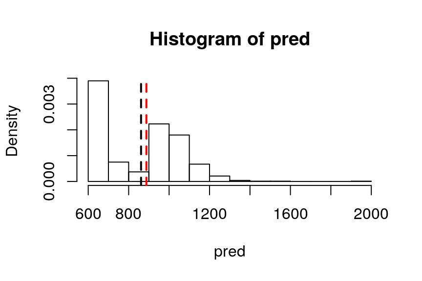
Figure 1 - Travel time distribution for trip ID 2700 for 1 000 runs using the test data set with an HMM model.
Model type comparison
Figure 2 shows the histograms of travel time for each of the four models for the same example.
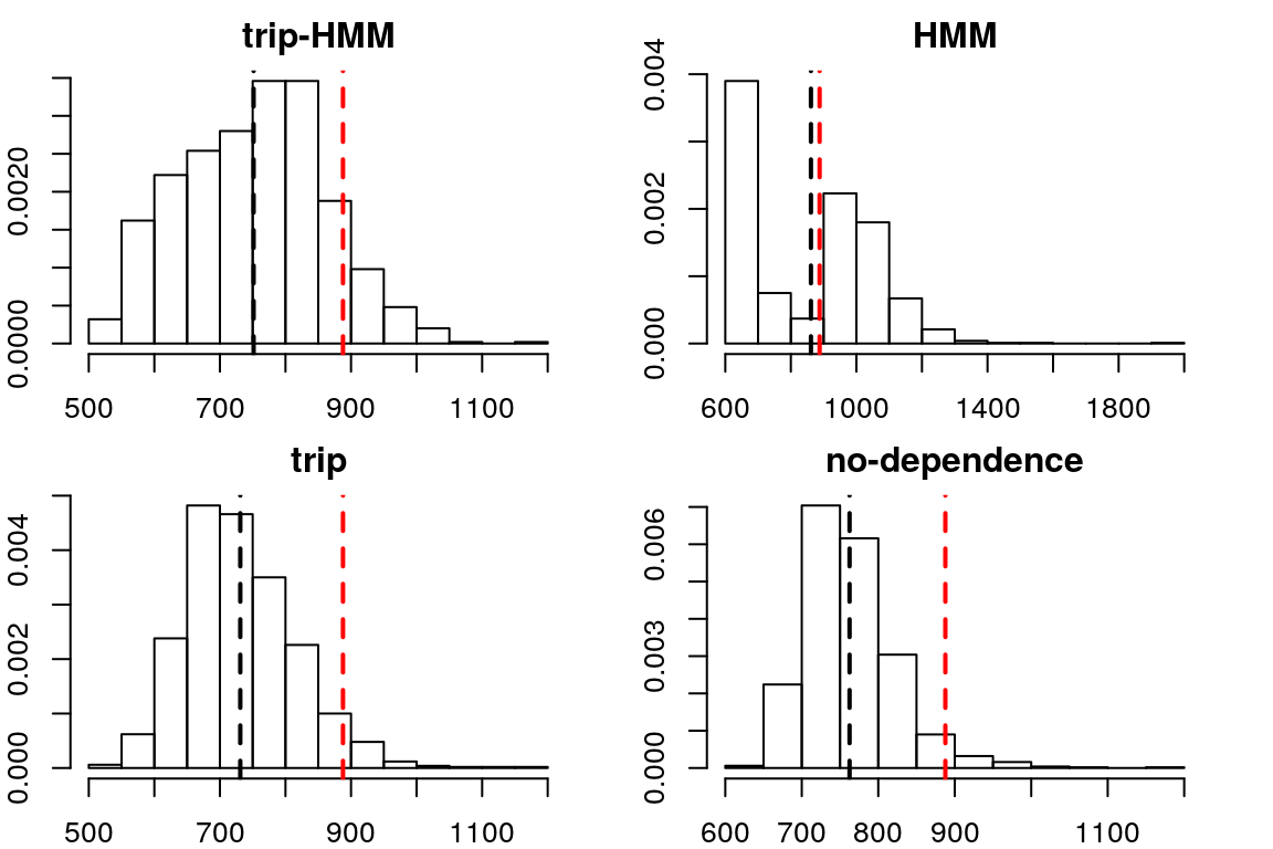
Figure 2 - Comparison of travel time distribution for the four model types for the same example.
Time bins
To specify different time bins than the ones supplied, traveltimeHMM provides a functional method called rules2timebins() that translates human readable weekly time bins to a conversion function.
rules2timebins() takes a list of lists of time bin rules, where each sub-list specifies 4 variables, start and endas the start and end time of a time bin in 24h format, days as a vector specifying the weekdays this time bin applies to, 1 for Sunday, and 2:5 for weekdays, and finally a tag to specify a name for the time bin.
For example,
rules = list(
    list(start='6:30',  end= '9:00',  days = 1:5, tag='MR'),
    list(start='15:00', end= '18:00', days = 2:5, tag='ER')
)
specifies two time bins calls MR for morning rush, and ER for evening rush, the former is for all weekdays and the latter is for Tuesdays to Fridays. All other time intervals are assigned a time bin called Other.
Passing rules to rules2timebins() would return an easy to use functional, for example
time_bins <- rules2timebins(rules)
time_bins("2019-08-16 15:25:00 EDT") ## Friday
[1] "ER"
time_bins("2019-08-17 21:25:58 EDT") ## Saturday
[1] "Other"
To change the time bins in tripset, run the code
tripset$timeBin <- time_bins(tripset$time)
head(tripset)
  tripID linkID timeBin logspeed traveltime    length                time
1   2700  10469   Other 1.692292  13.000000  70.61488 2014-04-28 06:07:27
2   2700  10444   Other 2.221321  18.927792 174.50487 2014-04-28 06:07:41
3   2700  10460   Other 2.203074   8.589937  77.76295 2014-04-28 06:07:58
4   2700  10462   Other 1.924290  14.619859 100.15015 2014-04-28 06:08:07
5   2700  10512   Other 1.804293   5.071986  30.81574 2014-04-28 06:08:21
6 2700 5890 Other 2.376925 31.585355 340.22893 2014-04-28 06:08:26Remark: at package loading a default time_bins() functional is created, which constructs the default time bins of tripset.
Prediction with new time bins
The estimation step traveltimeHMM does not utilize the new functional time_bins(), however in the prediction stage, predict requires input of the proper time bin functional. This can be seen by the arguments of predict as
where the argument time_bins.fun = time_bins is already specified to the default time_bins() functional. Hence, in prediction under a new time bin categories, the constructed functional must be passed as `time_bins.fun.
In the above example this would require refitting the data and re-predicting as
fit <- traveltimeHMM(data = tripset,nQ = 2,max.it = 20, model = "HMM")
#> Model HMM with 4914 trips over 13235 roads and 3 time bins...
#> Expected completion of 20 iterations in 116 secs
#> Reached maximum number of iterations


pred <- predict(object = fit, tripdata = single_trip,
                starttime = single_trip$time[1],
                n = 1000, time_bins.fun = time_bins)
hist(pred, freq=FALSE)
References
Woodard, D., Nogin, G., Koch, P., Racz, D., Goldszmidt, M., Horvitz, E., 2017. “Predicting travel time reliability using mobile phone GPS data”. Transportation Research Part C, 75, 30-44. http://dx.doi.org/10.1016/j.trc.2016.10.011